How to Graph CNV Data
opts_chunk$set(fig.width=8, fig.height=13)
#### make sure to load gUtils
library(gTrack)
#### load in SCNA data
#### these are level 3 segments from over 1600 TCGA breast cancer cases
#### downloaded from the TCGA and converted to a single GRanges object
scna = seg2gr(readRDS(gzcon(url("https://data.broadinstitute.org/snowman/gTrack/inst/extdata/files"))))

#### we define amplification events and deletion events
#### and then do a simple recurrence analysis on amplifications

#### amplification events are defined using %Q% gUtils operator to filter
#### on scna metadata for segments with seg.mean greater than 1
#### greater than 50 markers and width less than 1MB
 amps = scna %Q% (seg.mean>1 & num.mark > 50 & width < 1e7)

#### apply a similar filter to define deletions
 dels = scna %Q% (seg.mean<(-1) & num.mark > 50 & width < 1e7)

#### compute the amplification "score" as the total number of amplification
#### events in a given region
 amp.score = as(coverage(amps), 'GRanges')

#### define the peaks of amplification as the 100 regions with
#### the highest amplification score
 amp.peaks = amp.score %Q% (rev(order(score))) %Q% (1:100)

#### "reduce" or merge the top peaks to find areas of recurrent amplification
amp.peaks = reduce(amp.peaks+1e5) %$% amp.peaks %Q% (rev(order(score)))

### do a similar analysis for dels
del.score = as(coverage(dels), 'GRanges')
del.peaks = del.score %Q% (rev(order(score))) %Q% (1:100)
del.peaks = reduce(del.peaks+1e5) %$% del.peaks %Q% (rev(order(score)))

#### load in GRanges of GENCODE genes
genes = readRDS(system.file("extdata", 'genes.rds', package = "gTrack"))

#### use %$% operator to annotate merged amp and del peaks with "gene name" metadata
amp.peaks = amp.peaks %$% genes[, 'gene_name']
del.peaks = del.peaks %$% genes[, 'gene_name']

### now that we've computed scores and annotated peaks
### we want to inspect these peaks and plot them with gTrack

### load in precomputed gTrack of hg19 GENCODE annotation
### (note this is different from the GENCODE genes which is a GRanges
### we loaded in a previous line .. this is purely for visualization)
ge = track.gencode()
## Pulling gencode annotations from /data/research/mski_lab/Software/R/gTrack/extdata/gencode.composite.collapsed.rds
#### build a gTrack of amps colored in red with black border
#### and one of dels colored in blue
gt.amps = gTrack(amps, col = 'red', name = 'Amps')
gt.dels = gTrack(dels, col = 'blue', name = 'Dels')
#### build a gTrack of amp and del score as a line plot
gt.amp.score = gTrack(amp.score, y.field = 'score',
col = 'red', name = 'Amp score', line = TRUE)
gt.del.score = gTrack(del.score, y.field = 'score',
col = 'blue', name = 'Amp score', line = TRUE)
#### build a gTrack of peaks of amp and del peaks
gt.amp.peaks = gTrack(amp.peaks, gr.labelfield = 'gene_name',
col = 'pink', border = 'black', name = 'Amp peaks', height = 5)
gt.del.peaks = gTrack(del.peaks, gr.labelfield = 'gene_name',
col = 'lightblue', border = 'black', name = 'Amp peaks', height = 5)
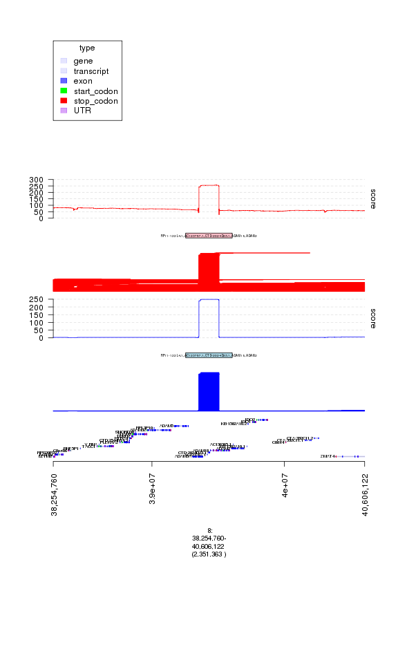
### let's look at the top amplification peak
amp.peaks[1]
## GRanges object with 1 range and 2 metadata columns:
##       seqnames               ranges strand |     score
##          <Rle>            <IRanges>  <Rle> | <numeric>
##   [1]        8 [39254760, 39606122]      * |  253.9448
##                                                    gene_name
##                                                  <character>
##   [1] RP11-122L4.1, AC123767.1, CTD-2024D23.1, ADAM18, ADAM2
##   -------
##   seqinfo: 24 sequences from an unspecified genome
### interesting! this looks like a novel peak with genes that have
### not previously been associated with breast cancer
### ("RP11-122L4.1, AC123767.1, CTD-2024D23.1, ADAM18, ADAM2")

### let's look at the data supporting this peak - including
### the underlying amp events, amp score, and peak region boundary
plot(c(ge, gt.amps, gt.amp.peaks, gt.amp.score), amp.peaks[1]+1e6)

plot of chunk plot1
### hmm, something looks suspicious since all the segments have the same
### start and end. These could be copy number artifacts that often arise
### in segmentation of array data, sometimes due to germline copy number
### polymorphisms.
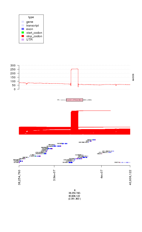
### to see this pattern more clearly, let's enlarge the
### amplification track, also add the deletion data, and replot
my.gt = c(ge, gt.dels, gt.del.peaks, gt.del.score,
gt.amps, gt.amp.peaks, gt.amp.score)
plot(my.gt, amp.peaks[1]+1e6)
plot of chunk plot2
### interesting so this appears to also be a peak in the deletion analysis
### and a region that accumulates both amplification and deletion calls in
### many tumor samples.  This could either be a copy number polymorphism
### or an artifact.

### let's load in a track of copy events from the Database of Germline Variation
### which catalogues common copy changes in human populations
dgv = readRDS(system.file(c('extdata/files'), 'dgv.rds', package = 'gTrack'))
plot(c(ge, gt.amps, gt.amp.peaks, gt.amp.score), amp.peaks[1]+1e6)
plot of chunk plot3
### indeed looks like this is a region around which people have previously
### seen germline copy number variations, so it's likely an artifact

### let's look at the next amp peak
print(amp.peaks[2])
## GRanges object with 1 range and 2 metadata columns:
##       seqnames               ranges strand |     score
##          <Rle>            <IRanges>  <Rle> | <numeric>
##   [1]       11 [68809874, 69577804]      * |  102.4002
##                                                                                                                                                     gene_name
##                                                                                                                                                   <character>
##   [1] TPCN2, MIR3164, RP11-554A11.7, RP11-554A11.8, MYEOV, RP11-211G23.2, RP11-211G23.1, AP000439.1, AP000439.2, AP000439.5, AP000439.3, CCND1, ORAOV1, FGF19
##   -------
##   seqinfo: 24 sequences from an unspecified genome
### this peak includes  CCND1 in addition to other genes
### this peak is known to be a target of amplification in breast cancer
### and so likely real

### let's plot it:
plot(my.gt, amp.peaks[2]+1e6)
## budget ..
## Error in (function (...) : all elements in '...' must be GRanges objects
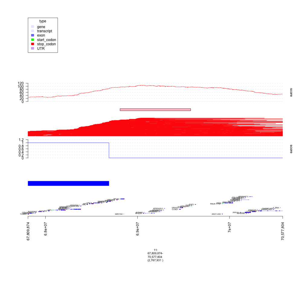
plot of chunk plot4
### unlike the previous peak this has an enrichment of amplifications vs deletions
### not known have a bunch of germline copy number changes in the DGV

### let's zoom in on the individual events, getting rid of the other tracks
### increase the height of the amp track
### and adding a black border to better define event boundaries
gt.amps$border = 'black'
gt.amps$height = 30
my.gt = c(ge, gt.amps, gt.amp.peaks, gt.amp.score)
plot(my.gt, amp.peaks[2]+1e6)
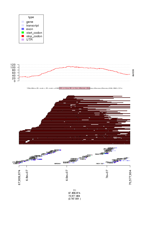
plot of chunk plot5
### here each red segment is a somatic amplification or gain in a different patietn
### the peak looks real, in that the events have relatively random starts
### and ends and cluster around this target gene.