How to Graph Structural Variations
## make sure to load in these libraries
library(gTrack)
library(bamUtils) ## to use read.bam function
options(warn=-1)
## this load sequences that have had coverage calculated from cancer cell lines (GRanges object, have to make into a gTrack)
cov = readRDS(gzcon(url('https://data.broadinstitute.org/snowman/gTrack/inst/extdata/coverage.rds')))

## wrap a gTrack around this, draw with blue circles, and label the track "Cov" and sets 0 as lower bound for all views
gt.cov = gTrack(cov, y.field = 'mean', circles = TRUE, col = 'blue', name = 'Cov')

## this loads the junctions data from the cell line (GRangesList, where each item is a length 2 GRanges
## with strand information specifying the two locations and strands that are being fused)
junctions = readRDS('../../inst/extdata/junctions.rds')

## loading the GENCODE gene model gTrack (hg19 pre-loaded comes with gTrack,
## but can be made from any .gff file from GENCODE (http://www.gencodegenes.org/releases/19.html)
gt.ge = track.gencode()
## Pulling gencode annotations from /Library/Frameworks/R.framework/Versions/3.3/Resources/library/gTrack/extdata/gencode.composite.collapsed.rds
## this loads a gTrack object of a genome graph i.e. network of the same cancer cell line (generated by JaBba)
graph = readRDS('../../inst/extdata/graph.rds')

## pick an interesting junction and plot the genes, coverage, and genome graph around it
## the links argument specifies the junctions that are being drawn
window = junctions[[290]] + 1e5
plot(c(gt.ge, gt.cov, graph), window, links = junctions)
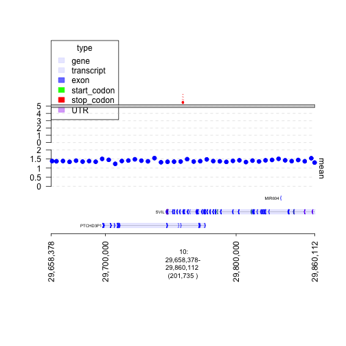
plot of chunk plot-firstSV
ix = 194
cwindow = junctions[[ix]]

jix = c(582, 583)
window = unlist(junctions[jix]) + 3e5

## convert junctions to a data frame. values() returns values from the hash which is the junctions object, in this example.
values(junctions)$col = 'gray'
values(junctions)$lwd = 1
values(junctions)$lty = 2 ## dashed instead of dotted line style
values(junctions)$col[jix] = 'red'
values(junctions)$lwd[jix] = 3 ## thicker line width
values(junctions)$lty[jix] = 1 ## solid line style for junction of interest
plot(c(gt.ge, gt.cov, graph), window, links = junctions)
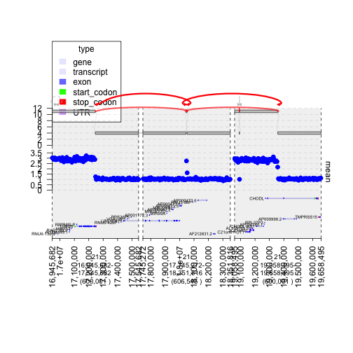
plot of chunk plot2ndgraph
Graping BAM data
## 4 windows corresponding to the 4 breakpoints involved in these two rearrangements.
window = unlist(junctions[jix]) + 250

## pull the reads out in these windows from the tumor and normal bam file.
treads = read.bam("../../inst/extdata/files/tumor.bam", window)
nreads = read.bam("../../inst/extdata/files/normal.bam", window)

## make them into gTracks
td.treads = gTrack(treads, draw.var = TRUE, name = 'Tumor reads')
td.nreads = gTrack(nreads, draw.var = TRUE, name = 'Normal reads')
plot(c(gt.ge, td.nreads, td.treads), window, links = junctions)
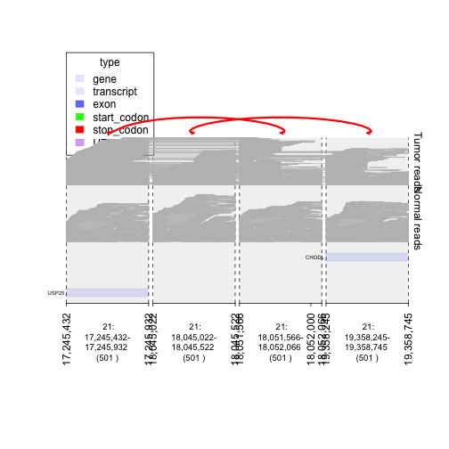
plot of chunk graph_BAM_data
## dividing tumor read pairs between those that support a rearrangement (i.e. hit multiple windows)
## and concordant read pairs that lie only within a single window
treadsr = treads[grl.in(treads, window, logical = FALSE)>1]
treadsc = treads[grl.in(treads, window, logical = FALSE)==1]

## isolating normal
nreadsr = nreads[grl.in(nreads, window, logical = FALSE)>1]
nreadsc = nreads[grl.in(nreads, window, logical = FALSE)==1]

td.treadsr = gTrack(treadsr, draw.var = TRUE, name = 'Tumor reads R', height = 30, angle = 45)
td.nreadsr = gTrack(nreadsr, draw.var = TRUE, name = 'Normal reads')
td.treadsc = gTrack(treadsc, draw.var = TRUE, name = 'Tumor reads')
td.nreadsc = gTrack(nreadsc, draw.var = TRUE, name = 'Normal reads C')
plot(c(gt.ge, td.nreadsc, td.nreadsr, td.treadsc, td.treadsr), window, links = junctions)
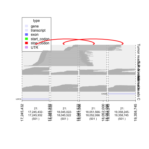
plot of chunk plotingTumors