How to Create Graphs¶

During chromosomal rearrangements, translocations may occur and graphing such a phenomenon is possible with gTrack. However, the edges parameter must be used. This vignette will explain how to prepare a graph.

Edges Parameter¶

In order to create a connected graph in gTrack, the edges parameter of gTrack must be supplied a matrix or a data frame of connections.

##create a GRanges object storing 10 sequences. These sequences will serve as nodes for the graph.
gr <- GRanges(seqnames = Rle(c("chr1" , "chr2" , "chr1" , "chr3") ,
  c(1,3,2,4)), ranges = IRanges(c(1,3,5,7,9,11,13,15,17,19) ,
  end = c(2,4,6,8,10,12,14,16,18,20),
  names = head(letters,10)),
  GC=seq(1,10,length=10),
  name=seq(5,10,length=10))

gr

## GRanges object with 10 ranges and 2 metadata columns:
##     seqnames    ranges strand |        GC             name
##        <Rle> <IRanges>  <Rle> | <numeric>        <numeric>
##   a     chr1  [ 1,  2]      * |         1                5
##   b     chr2  [ 3,  4]      * |         2 5.55555555555556
##   c     chr2  [ 5,  6]      * |         3 6.11111111111111
##   d     chr2  [ 7,  8]      * |         4 6.66666666666667
##   e     chr1  [ 9, 10]      * |         5 7.22222222222222
##   f     chr1  [11, 12]      * |         6 7.77777777777778
##   g     chr3  [13, 14]      * |         7 8.33333333333333
##   h     chr3  [15, 16]      * |         8 8.88888888888889
##   i     chr3  [17, 18]      * |         9 9.44444444444444
##   j     chr3  [19, 20]      * |        10               10
##   -------
##   seqinfo: 3 sequences from an unspecified genome; no seqlengths

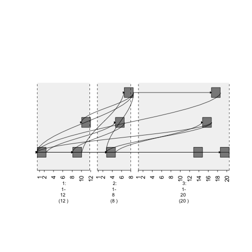
## Specify links between nodes using a matrix. Numeric 1s refer to a connection while conversely with 0s.

##create an N*N matrix filled with 0s.
graph = matrix(0 , nrow = 10 , ncol = 10)

##set certain indices to 1.
graph[1,3]=1
graph[1,10]=1
graph[2,5]=1
graph[2,8]=1
graph[3,5]=1
graph[4,1]=1
graph[4,2]=1
graph[4,6]=1
graph[4,9]=1
graph[5,1]=1
graph[5,2]=1
graph[5,4]=1
graph[8,1]=1
graph[8,2]=1
graph[9,1]=1
graph[10,1]=1

##use edges parameter to create graph.
plot(gTrack(gr , edges = graph , stack.gap = 5))

plot of chunk plot1

col Column¶

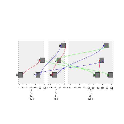
If a matrix is used to create a graph, color and style of edges cannot be specified.Instead of using a matrix, a data frame can be used to specify those attributes.

##the "from" column specifies the beginning node (range).
##the "to" column specifies the end node (range).
##the "col" specifies the color of the edge.
graph = data.frame(from = 1:9, to = c(6,9,7,2,4,10,8,5,3) , col = c('red', 'blue', 'green'))

plot(gTrack(gr , edges = graph , stack.gap = 5))

plot of chunk colored-graph

lwd Column¶

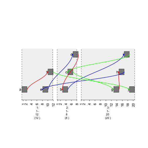
To change the width of the edges, use the lwd parameter.

##the "lwd" column specifies the width of the edge.
 graph$lwd = 1.844941
 graph

##   from to   col      lwd
## 1    1  6   red 1.844941
## 2    2  9  blue 1.844941
## 3    3  7 green 1.844941
## 4    4  2   red 1.844941
## 5    5  4  blue 1.844941
## 6    6 10 green 1.844941
## 7    7  8   red 1.844941
## 8    8  5  blue 1.844941
## 9    9  3 green 1.844941

plot(gTrack(gr, edges = graph, stack.gap = 5))

plot of chunk width-graph

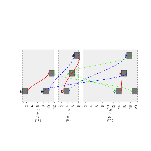
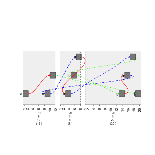
lty Column¶

Change style of edge by lty parameter.

## lty specifies the style of the edge (no dashes, big dashes, little dashes)
graph$lty = c(1,2,3)

plot(gTrack(gr , edges = graph , stack.gap = 5))

plot of chunk style-graph

h Column¶

Increase “curviness” of the edges by adding h column.

graph$h = 10

plot(gTrack(gr , edges = graph , stack.gap = 5))

plot of chunk curviness-graph